Matplotlib: Seeing Your Data
Numbers hide things. Pictures do not.
Here are the thali orders from Meera's kitchen for one week: 310, 295, 320, 305, 340, 260, 150. Look at them for a second. What is going on?
You can work it out, but it takes effort. Now look at the same seven numbers as a line:
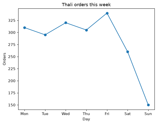
Weekdays are steady, Friday is the busiest, and the weekend falls off a cliff. You saw that in about one second. That is why every ML project starts by drawing the data, and Matplotlib is the library almost everyone uses to do it.
Your first chart
This is the exact code that drew the chart above:
1import matplotlib.pyplot as plt
2
3days   = ["Mon", "Tue", "Wed", "Thu", "Fri", "Sat", "Sun"]
4orders = [310, 295, 320, 305, 340, 260, 150]
5
6plt.plot(days, orders, marker="o")
7plt.title("Thali orders this week")
8plt.xlabel("Day")
9plt.ylabel("Orders")
10plt.show()
Every chart in Matplotlib follows the same pattern, so it is worth reading line by line:
Key Points
- import matplotlib.pyplot as plt: the usual import, with the usual nickname plt.
- plt.plot(days, orders): draw a line. The first list goes along the bottom (the x-axis), the second goes up the side (the y-axis). marker="o" puts a dot on each point.
- plt.title, plt.xlabel, plt.ylabel: a heading and labels for both axes.
- plt.show(): display the chart.
Tip:Get into the habit now: every chart gets a title and labelled axes. A chart without labels makes the reader guess what they are looking at, and six months later that reader might be you.
Four charts cover almost everything
There are dozens of chart types, but in everyday ML work you will use four of them most of the time. The trick is knowing which question each one answers:
Key Points
- Line chart: how does something change over time?
- Bar chart: how do different groups compare?
- Scatter plot: are two numbers related?
- Histogram: how are the values spread out?
You have seen the line chart. For the other three we will use the Pune flats data from the pandas lesson. Load it first:
1import pandas as pd
2import matplotlib.pyplot as plt
3
4df = pd.read_csv("https://cod-e.vercel.app/data/pune-flats.csv")
Bar chart: comparing groups
In the pandas lesson you worked out the average rent for each area as a list of numbers. As a bar chart:
1avg_rent = df.groupby("area")["rent"].mean().sort_values()
2
3plt.barh(avg_rent.index, avg_rent.values)
4plt.title("Average rent by area")
5plt.xlabel("Rent (₹ per month)")
6plt.show()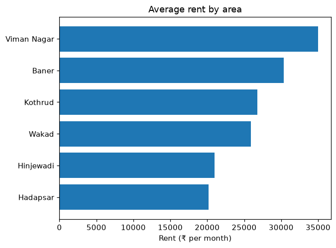
We used barh, which draws the bars sideways. Area names are long, and sideways bars give them room instead of squashing them together along the bottom. Sorting first puts the bars in order, which makes the chart far easier to read.
Scatter plot: are two things related?
This is the most important chart for machine learning. It puts one dot per row, with one number across and another number up. Here, every dot is a flat:
1plt.scatter(df["size_sqft"], df["rent"])
2plt.title("Bigger flats cost more")
3plt.xlabel("Size (sq ft)")
4plt.ylabel("Rent (₹ per month)")
5plt.show()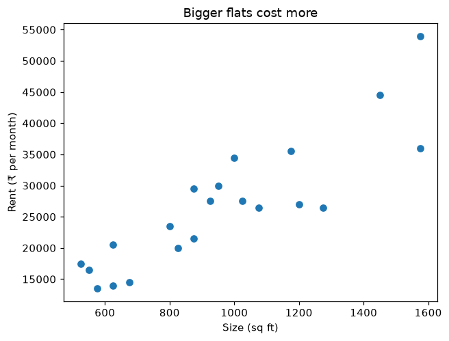
The dots drift from bottom left to top right. That tells you size and rent are related, so size will be a useful feature for predicting rent. Remember the three checks for a good feature in lesson 1.6? A scatter plot is how you test the first one: is it related to the target?
But the dots are not a perfect line. Some flats of the same size rent for very different amounts. Something else matters too. Let us colour the dots by furnishing:
1furnished   = df[df["furnished"] == "yes"]
2unfurnished = df[df["furnished"] == "no"]
3
4plt.scatter(furnished["size_sqft"], furnished["rent"], label="furnished")
5plt.scatter(unfurnished["size_sqft"], unfurnished["rent"], label="unfurnished")
6plt.title("Size vs rent, split by furnishing")
7plt.xlabel("Size (sq ft)")
8plt.ylabel("Rent (₹ per month)")
9plt.legend()
10plt.show()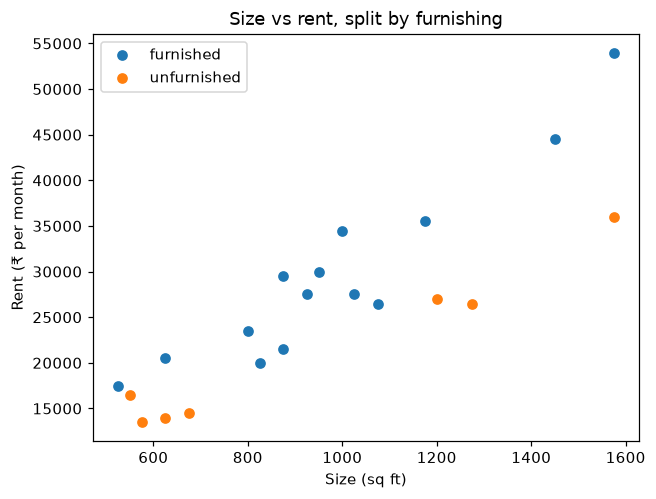
Now a second pattern appears. At almost every size, the furnished flats sit higher than the unfurnished ones. We filtered the data into two groups with pandas, drew both on the same chart, and label plus plt.legend() added the little key in the corner.
This is real ML thinking. You have just discovered, by looking, that a model predicting rent should know about furnishing as well as size.
Histogram: how values are spread out
A histogram answers a different question: are most rents cheap, expensive, or somewhere in the middle? It splits the range of rents into equal slices, called bins, and counts how many flats fall into each one:
1plt.hist(df["rent"], bins=8)
2plt.title("How rents are spread out")
3plt.xlabel("Rent (₹ per month)")
4plt.ylabel("Number of flats")
5plt.show()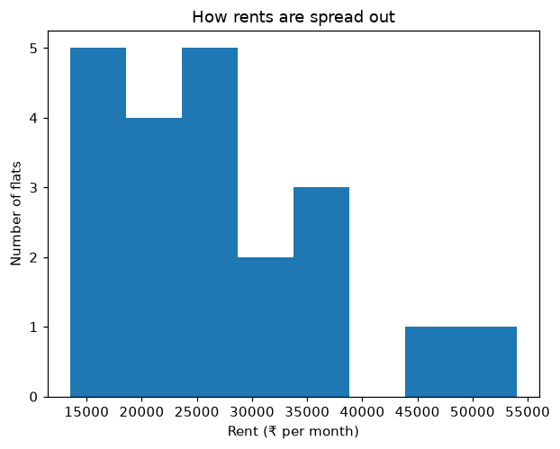
Most flats are bunched on the left, between about ₹13,500 and ₹38,000. Then there is a gap, and two expensive flats sit far out on the right. That shape, a big bunch with a long tail on one side, is very common in real data like prices and salaries. It matters a lot for the statistics lesson coming up.
Tip:Our dataset only has 21 flats, so the histogram looks lumpy. With thousands of rows, histograms turn into smooth shapes. Try changing bins=8 to bins=4 or bins=15 and see how the picture changes.
A shortcut from pandas
pandas can call Matplotlib for you, straight from a DataFrame. This one line draws the same scatter plot as before:
1df.plot(kind="scatter", x="size_sqft", y="rent", title="Bigger flats cost more")Change kind to "hist", "bar" or "line" for the others. It is great for a quick look while exploring. When you want full control over how a chart looks, use plt directly, as in the rest of this lesson.
Charts can mislead
One warning before you go. Here are the average rents for Hadapsar (₹20,167) and Hinjewadi (₹21,000), drawn twice:
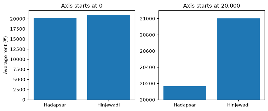
On the left, the bars are almost the same height, which is the truth: Hinjewadi is only about 4% more expensive. On the right, the axis starts at 20,000 instead of 0, and suddenly Hinjewadi looks about six times pricier.
Nothing on the right is technically false. The numbers are the same. But it tells a different story. Always check where the axis starts, both on charts you make and on charts other people show you. Bar charts should almost always start at zero.
Where people get confused
Key Points
- "Charts are just for presentations at the end." In ML, charts are a thinking tool. You draw them at the start, to understand the data before building anything.
- "The first list in plt.plot goes up the side." The first goes along the bottom (x-axis), the second goes up the side (y-axis).
- "A bar chart and a histogram are the same thing." A bar chart compares separate groups, like areas. A histogram shows how one set of numbers is spread across ranges.
- "The chart did not appear." In a script you need plt.show(). In Colab, charts usually appear anyway, but writing plt.show() is a good habit.
Quick check
You want to know whether study hours are related to exam marks. Which chart?
A scatter plot, with study hours along the bottom and marks up the side. If the dots drift up to the right, more study goes with higher marks.
You want to compare the number of orders from each of five cities. Which chart?
A bar chart, one bar per city. It compares separate groups.
A news channel shows a bar chart where one party's bar is three times taller than another's. What should you check first?
Where the vertical axis starts. If it does not start at zero, a small real difference can be made to look huge.
Recap
Key Points
- Pictures reveal patterns in seconds that are hard to see in a table of numbers.
- The pattern: plt.something(...), then a title and axis labels, then plt.show().
- Line for change over time, bar for comparing groups, scatter for relationships, histogram for spread.
- Scatter plots are how you check whether a feature is related to the target.
- Check where the axis starts. Bar charts should start at zero.
Next up: scikit-learn. You have trained a few models with it already. Now let us see how it is organised, and why every model in it works the same way.
Theia
Can you explain this concept?
Practise Matplotlib: Seeing Your Data with realistic interview questions. Choose spoken or typed answers, get feedback on your reasoning, then return to the material that needs work.
Sign in to practise this conceptThe session stays focused on this lesson. Your selected interview level sets the bar.